In Chap. 10, we investigated various beta diversity metrics and ordination techniques. This chapter will continue to contribute to beta diversity. First, we describe the general nonparametric methods for multivariate analysis of variance in ecological and microbiome data (Sect. 11.1). Then, we mainly introduce two statistical hypothesis tests of beta diversity: analysis of similarity (ANOSIM) and permutational MANOVA (PERMANOVA) in Sects. 11.2 and 11.3, respectively. Next, we introduce analysis of multivariate homogeneity of group dispersions (Sect. 11.4). Section 11.5 introduces pairwise PERMANOVA. Section 11.6 introduces how to identify core microbial taxa. Section 11.7 describes statistical testing of beta diversity in QIIME 2. Finally, we briefly summarize this chapter in Sect. 11.8.
11.1 Introduction to Nonparametric MANOVA Using Permutation Tests
In Chap. 10 (Sect. 10.3.9.1), we reviewed that CCA (ter Braak 1986) ushered in the biggest modern revolution in ordination methods because it makes ordination to be not mere an “exploratory” method, but also a hypothesis testing method. Still an important advance in the analysis of multivariate data in ecology was the development of nonparametric methods for testing hypotheses concerning whole communities, particularly by using permutation techniques, such as works from Clarke (1988, 1993), Smith et al. (1990), and Biondini et al. (1991). The importance of testing hypotheses in multivariate analyses in ecology has been reviewed by Anderson (2001). As Anderson stated, before the development of nonparametric methods for testing hypotheses, particularly ANOSIM (Clarke 1993), the most widely available multivariate analyses in ecology focused on the reduction of dimensionality: either to produce and interpret patterns (ordination methods) or to place observations into natural groups by using numerical strategies (clustering). However, although “any inference from the particular to the general must be attended with some degree of uncertainty,” “the mathematical attitude toward induction” is still rigorous in the sense that the degree of uncertainty can be expressed in terms of mathematical probability (Fisher 1971; Anderson 2001). In terms of mathematical probability, ordination and clustering methods do not rigorously express the nature and degree of uncertainty concerning a priori hypotheses; it is methods like Mantel’s test (Mantel 1967), ANOSIM (Clarke 1993), and multi-response permutation procedures (Mielke Jr. et al. 1976) that allow such rigorous probabilistic statements to be made for multivariate ecological data (Anderson 2001).
The starting point of nonparametric methods for testing hypotheses is to use an analysis-of-variance approach and nonparametric techniques (permutation tests), but minimize the statistical assumptions about the data or be free of the assumption of multivariate normality required by parametric MANOVA. The minimized or less stringent primary statistical assumption is that the data are independently and identically distributed (exchangeability of replicates) (Legendre and Anderson 1999; Anderson 2001).
In the remaining of this chapter, we introduce statistical hypothesis testing of beta diversities through nonparametric MANOVA tests and other related nonparametric methods.
11.2 Analysis of Similarity (ANOSIM)
ANOSIM was developed under a unified framework (Clarke 1993) to (1) display the community patterns through clustering and ordination of samples, (2) identify the species principally responsible for determining sample groupings, (3) perform statistical tests for differences in space and time (analogues of parametric MANOVA, based on rank similarities), and (4) link the community differences to patterns in the environment (also dictated by rank similarities between samples). ANOSIM focuses on hypothesis testing, which is the third component of this framework.
ANOSIM is a nonparametric multivariate statistical method for analysis of changes in community structure based on a standardized rank correlation between two distance matrices. ANOSIM was developed under above described unified framework (Clarke 1993). As a distribution-free method of multivariate data analysis, ANOSIM is frequently used by community ecologists and microbiome researchers.
11.2.1 Introduction of ANOSIM
Clarke (1993) proposed a nonparametric method called “analysis of similarities” (ANOSIM) test to perform the null hypothesis testing of “no differences between sites (groups)” by permutations of the rank similarity matrix. Clarke (1993) thought that rank similarities among samples play a fundamental role in defining and visualizing the community pattern because of the following: (1) Generally relative levels and in particular the ranks of the similarity matrix have a natural interpretation, in which the ranks of similarity matrix summarize the data through statements such as “sample A is more similar to sample B than it is to sample C.” (2) The rank similarity is intuitively appealing and very generally applicable to build a graphical representation of the sample patterns. (3) Particularly in effect, this is the only information that a successful NMDS ordination used.
ANOSIM is a nonparametric one-way ANOVA procedure for testing the hypothesis of no difference based on permutation test of the corresponding (rank) similarities among- and within-group samples in the underlying triangular similarity matrix (Clarke 1993). Like ANOVA, ANOSIM treats group membership or treatment levels as factors and models them as the explanatory variable. Analysis of similarity is based on the simple idea: if the tested groups are meaningful, then samples within the groups should be more similar in composition than samples from different groups. The test statistic is given below:

 is the mean of rank similarities from all pairs of samples between different groups.
 is the mean of all rank similarities among samples within groups.
M = n(n − 1)/2 and n is the total number of samples under consideration.
Step 1: calculate dissimilarity matrix.
Step 2: calculate rank dissimilarities and assign a rank of 1 to the smallest dissimilarity.
Step 3: calculate the mean among- and within-group rank dissimilarities.
Step 4: calculate test statistic R using the above formula
 .
.That is, the value of R taken is calculated based on the similarities only for the individual groups (sites), extracted from the matrix for all groups (sites) and re-ranked.
Step 5: test for significance. As in PERMANOVA test (see Sect. 11.3.1), the P-value of test statistic R is obtained by permutation: randomly assigning sample observations to groups. Then, the ranked similarity within and between groups is compared with the similarity that would be generated by random chance. The significance test is simply the fraction of permuted R’s that are greater than the observed value of R. That is, it is the probability of an R given this large or larger. Under the null hypothesis H0, “no differences between groups (sites),” there will be little effect on average to the value of R if the labels identifying which samples (replicates) belong to which groups (sites) are arbitrarily rearranged (Clarke 1993); that is, the total samples from all groups (sites) are just replicates from a single group (site) if H0 is true. The rationale for a permutation test of H0 is to examine all possible allocations of labels per group (site) to the total samples and recalculate the R statistic for each. The algorithm behind the hypothesis testing is same as PERMANOVA: if two groups of sampling units are really different in their species (or other taxa) composition, then compositional dissimilarities between the groups ought to be greater than those within the groups (see details in Sect. 11.3.1).
In this test statistic, the highest similarity is assigned to a rank of 1 (the lowest value).
R lies in the range (−1, 1).
R = 1 only if all samples within groups are more similar to each other than any samples from different groups.
R = 0 if the null hypothesis is true, which suggests that similarities between and within groups are the same on average.
R will usually fall between 0 and 1, indicating some degree of discrimination between the groups.
If the null hypothesis is rejected, then R ≠ 0, which suggests that all pairs of samples within groups are more similar than to any pair of samples from different groups. For example, in the case all the most similar samples are within the sample groups, then R = 1. Theoretically, it is also possible that R < 0, but practically such case is unlikely in ecological and microbiome studies; such an occurrence is more likely to indicate an incorrect labeling of samples. The extreme case is R = −1, which indicates that the most similar samples are all not in the groups.
11.2.2 Perform ANOSIM Using the Vegan Package
ANOSIM provides a way to statistically test whether there is a significant difference between two or more groups of sampling units. ANOSIM is implemented via the function anosim() in the vegan package. The function assumes that all ranked dissimilarities within groups have about equal median and range. The anosim() function requires a dissimilarity matrix as input data, which can be produced by the function dist() or vegdist(). A summary and plot methods are also available in ANOSIM to perform the post modeling analysis.
One syntax is given below:
data is data matrix or data frame in which rows are samples and columns are response variable(s), or a dissimilarity object or a symmetric square matrix of dissimilarities.
grouping is the grouping variable (a factor).
permutations is the number of permutations to assess the significance of the ANOSIM statistic.
distance is used to specify distance metric that measures the dissimilarity between two observations. When the input data is not a dissimilarity structure or a symmetric square matrix, then this argument needs to be specified.
strata is an integer vector or factor which is used for specifying the strata for permutation. If supplied, observations are permuted only within the specified strata.
In this section, we illustrate ANOSIM test using the same breast cancer QTRT1 mouse gut microbiome dataset (Jilei Zhang et al. 2020). We perform ANOSIM test using the following steps.
Step 1: Load otu table into R or RStudio.
Step 2: Make the dataset to have rows being samples and columns being OTUs.
The anosim() function requires the input data matrix or data frame in which rows are samples and columns are OTUs (taxa). Here, the dataset with rows is OTUs and columns being samples:
Thus, we transform the “abund_tab” to the “abund_tab_t” in which rows are samples and columns are OTUs:
Step 3: Perform ANOSIM tests of measures of dissimilarity.
Fit ANOSIM to test the Bray-Curtis dissimilarity.
Fit ANOSIM to test the Jaccard dissimilarity.
Partial output of binary Jaccard dissimilarity is given below:
Fit ANOSIM to test the Sørensen dissimilarity.
Step 4: Plot the dissimilarity ranks between and within groups.
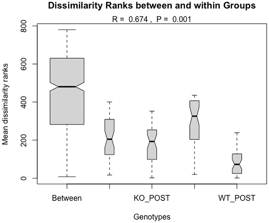
A graph of genotypes versus mean dissimilarity ranks. The title is dissimilarity ranks between and within groups. The genotypes are Between, K O POST, and W T POST. The values include R equals 0.674 and P equals 0.001.
Boxplot of Bray-Curtis dissimilarity based on QTRT1 mouse dataset
11.2.3 Remarks on ANOSIM
As described above, before the development of nonparametric methods for testing hypotheses, particularly ANOSIM (Clarke 1993), the most widely available multivariate analyses in ecology focused on ordination and clustering (the methods for reduction of dimensionality). The importance of ANOSIM lies on these three factors (Clarke 1993): (1) It emphasizes it is relevant ecological assumptions that dictate the choice of dissimilarity measure but not the mechanics of the ordination method. (2) It not only avoids the difficulty of choosing measures and even the ordination technique itself but also does not need to consider whether species-environment relationships may be linear, monotonic, unimodal, or even multimodal forms (Clarke 1993). In practice all four combinations may be present. Canonical analysis has been proposed to avoid constraining species-environment relationships to linear, monotonic, unimodal, or multimodal forms. However, it remains unknown how well it stands up to further detailed scrutiny. The direct hypothesis testing approach of ANOSIM is more appealing. (3) The third is simplicity and validity of advocated nonparametric techniques.
As we remarked in Chap. 10 (Sect. 10.1.3.1), because Sørensen dissimilarity and Jaccard dissimilarity are similarly defined and due to ANOSIM rank-based testing property, the testing results of Jaccard dissimilarity and the Sørensen dissimilarity are almost identical in this example. The result of Bray-Curtis dissimilarity has been reported in previous publication (Jilei Zhang et al. 2020). We also compared the effects of normalization with fitting ANOSIM using relative abundance and absolute count data. The results showed that normalization has no large effect for Jaccard dissimilarity and the Sørensen dissimilarity, which may be due to their binary property. Their results including distance measures and statistical tests are almost identical (only upper quantiles of permutations are different) in this case. However, for Bray-Curtis dissimilarity, the relative abundance data returned much larger distance values than using absolute count data. The relative abundance data also give a smaller R statistic compared to using absolute count data (0.613 vs. 0.674).
11.3 Permutational MANOVA (PERMANOVA)
In this section, we first describe how PERMANOVA was developed, and next illustrate how to conduct PERMANOVA in microbiome data, and then briefly remark on this method.
11.3.1 Introduction to PERMANOVA
In 2001, Anderson (2001) proposed a nonparametric method for multivariate analysis of variance based on permutation tests called “nonparametric MANOVA,” a permutational multivariate analysis of variance (PERMANOVA). PERMANOVA is used to perform the general multivariate null hypothesis of no differences in the composition and/or relative abundances of different species (taxa/variables) between two or more groups of samples.
PERMANOVA improves the previous nonparametric methods because it can be based on any measure of dissimilarity and by allowing a direct additive partitioning of variation for a multifactorial ANOVA model, while maintaining the flexibility of other nonparametric methods but lacking their formal assumptions. The test statistic is a multivariate analogue to Fisher’s F-ratio and is calculated directly from any symmetric distance or dissimilarity matrix. P-values are obtained using permutations.
Before PERMANOVA, many nonparametric MANOVA-like methods for tests of differences among a priori groups of observations have been developed, including Mantel (1967); Mantel and Valand (1970); Mielke Jr. et al. (1976); Clarke (1988, 1993); and Legendre and Anderson (1999).
All these methods generally share two things (Anderson 2001): (1) They are based on measures of distance or dissimilarity between pairs of individual multivariate observations (refer to generally as distances) or their ranks and construct a statistic to compare these distances among observations in the same group versus those in different groups, following the conceptual framework of ANOVA. (2) They use permutations of the observations to obtain a probability associated with the null hypothesis of no differences among groups. However, previous nonparametric MANOVA-like methods have been reviewed suffering three weaknesses (Anderson 2001): The main drawback to all these methods is that they are not able to cope with multifactorial ANOVA to partition variation across the many factors that form part of the experimental design (Anderson 2001). Thus, they had to take multiple one-way analyses and qualitative interpretations of ordination plots to infer interactions or variability at different spatial scales. Some of these methods do allow partitioning for a complex design, but are restricted for use with metric distance measures (i.e., Euclidean distance), instead of using the semimetric Bray-Curtis measure of ecological distance which is ideal for ecological applications. Furthermore, these methods lack of appropriate permutational strategies for complex ANOVA, particularly for tests of interactions and directly statistical analysis of Bray-Curtis distances for any multifactorial ANOVA design.
Step 1: Develop an F-ratio test statistic.
PERMANOVA is formulated based on the analysis and partitioning sums of square distance or dissimilarity matrix.
Let’s consider a matrix of distances between every pair of observations and let N = an, the total number of observations (points), and dij be the distance between observation i = 1, …, N and observation j = 1, …, N; then the total sum of squares SST is given below:

That is, add up the squares of all of the distances in the sub-diagonal (or upper-diagonal) half of the distance matrix (but not including the diagonal) and divide by N. SST is used to calculate average distance among all samples. Similarly, the within-group or residual sum of squares is given below:


The rationale for this test statistics lies in the fact if the points from different groups have different central locations (centroids in the case of Euclidean distances) in multivariate space, then the among-group distances will be relatively large compared to the within-group distances, and the resulting pseudo-F-ratio will be relatively large.
Step 2: Obtain a P-value using permutations.
From Eq. (11.4), we can see that the bigger the ratio between SSA/(a − 1) and SSW/(N − a) (called the signal-to-noise ratio), the larger the F-value, and thus it results in a smaller P-value. The question is: how can we obtain a P-value? The individual variables in ecology and microbiome are typically not normally distributed, and we do not expect that the Euclidean distance will necessarily be used for the analysis. As Anderson (2001) observed, even if each of the variables were normally distributed and the Euclidean distance can be used, the mean squares calculated for the multivariate data would not each consist of sums of independent χ2 variables, because, although individual observations are expected to be independent, individual species (OTUs or taxa) variables are not independent of one another. Thus, traditional tabled P-values cannot be used.
Anderson (2001) proposed to create a distribution of the statistic under the null hypothesis using permutations of the observations (Edgington 1995; Manly 1997). The algorithm underlying this is that under the null hypothesis, the groups are not really different in terms of their composition and/or their relative abundances of species, as measured (e.g., by the Bray-Curtis distances); then the multivariate observations (rows) would be exchangeable among the different groups. Thus, we can randomly shuffle (permute) the rows that are identified to a particular group to obtain a new F-value (say, F*). The random shuffling is repeated and the F* is recalculated for all possible re-orderings of the rows. In such way, the entire empirical distribution of the pseudo-F-statistic under a true null hypothesis for the particular data is generated.
A P-value, which indicates the significance between groups, is calculated by comparing the F-value obtained with the original ordering of the rows to the empirical distribution created for a true null by permuting the labeled rows:

In general there are distinct ways of permuting the labels for n replicates at each of k sites (Clarke 1993). Although examining such a number of re-labeling is computationally possible and the precision of the P-value will increase with increasing numbers of permutations, however, the scale of calculation can quickly get out of hand with modest increases in replication. Thus, in practice it is usually not to calculate all possible permutations due to the time; P-value can be calculated using a large random subset of all possible permutations (Hope 1968), that is, usually is randomly sampled (with replacement). Generally, at least 1000 permutations are required for tests at a significance level of α = 0.05 and at least 5000 permutations for tests with a significance level of α = 0.01 (Manly 1997).
As presented above, permutations mean randomly assigning sample observations to groups. The P-value is calculated by comparing the permuted F-ratios to the observed F-ratio. The significance test is simply the fraction of permuted F-ratios that are greater than the observed F-ratio. Briefly, we can take one-way test as an example to explain what permutations actually do. In a one-way test, our interest is to see whether a statistic is either less than or greater than what can be expected by chance. The P-value is calculated from the proportion of permuted pseudo-F-statistics which are greater than or equal to the observed F-statistic. In another words, we want to know whether the permuted datasets following the PERMANOVA yield a better resolution of groups relative to the actual dataset. If more than 5% of the permuted F-statistics has values greater than that of the observed F-statistic, the P-value is greater than 0.05. Then, we can conclude that any difference among groups is not statistically significant.
11.3.2 Perform PERMANOVA Using the Vegan Package
We can perform PERMANOVA through the functions adonis() and adonis2() in the vegan package. These two functions analyze and partition the sums of squares using distance/dissimilarity matrices and fit linear models (e.g., factors, polynomial regression) to distance matrices using a permutation test with pseudo-F-ratios.
The adonis() and adonis2() functions are directly based on the algorithms of Anderson (2001) to perform a sequential test of terms and McArdle and Anderson (2001) to perform sequential, marginal, and overall tests, respectively. Both functions can handle semimetric indices (e.g., Bray-Curtis dissimilarity) that produce negative eigenvalues. The adonis2() also allows using additive constants or square root of dissimilarities to avoid negative eigenvalues (Stevens and Oksanen 2020). If the random permutation is the same, the adonis() and adonis2() will provide the identical results of tests. However, adonis2() could be much slower compared to adonis(), in particular when several terms are in the model (Stevens and Oksanen 2020).
ADONIS (permutational multivariate analysis of variance using distance matrices) method is less sensitive to dispersion effects (different within-group variation) and flexible than both ANOSIM (Clarke 1993) and multi-response permutation procedure (MRPP) (Mielke Jr. et al. 1976), which only handle categorical predictors (Oksanen 2016). ADONIS allows ANOVA-like tests of the variance in beta diversity explained by continuous and/or categorical predictors, which is a recommended method in the vegan package.
In general, ADONIS can be used to analyze ecological and microbiome community data as well as genetic data. The formers typically are samples by taxa matrices, while genetic data often have thousands or millions of columns of gene expression with a limited number of samples of individuals. Since ADONIS method is to perform PERMANOVA (permutational multivariate analysis of variance) using distance matrices, thus a distance/dissimilarity measure is required when running PERMANOVA (ADONIS). In microbiome literature, four beta diversity measures, Bray-Curtis distance, Jaccard distance, and weighted and unweighted UniFrac distances, have often been reported (Linnenbrink et al. 2013), and “bray” (the Bray-Curtis distance) has been most widely used.
One example syntax of adonis() is given as below:
formula = model formula, e.g., Y = A + B + C*D; Y must be either a community data matrix (data frame) or a dissimilarity matrix (data frame), e.g., inheriting from class “vegdist” or “dist”. If Y is a community data matrix, the function vegdist() will be used to calculate pairwise distances/dissimilarities. A, B, C, and D are the independent variables, which may be factors or continuous variables. They can be transformed within the formula.
data = the data frame for the independent variables.
permutations = 999 is the specified number of replicate permutations used for the hypothesis tests (F tests).
method = ““can be any method name used in the function vegdist () to calculate pairwise distances if the left-hand side of the formula is a data frame or a matrix.
contr.unordered = ““is used for contrasts of the design matrix; in general, R default uses dummy or treatment contrasts for unordered factors. However, the default contrasts in vegan package are different; they use “sum” or “ANOVA” contrasts.
contr.ordered = ““is used for contrasts of the design matrix for ordered factors.
One example syntax of adonis2() is given as below:
sqrt.dist = FALSE defines not to take square root of dissimilarities.
by = “terms” is set to assess significance for each term (sequentially from first to last), setting by = “margin” will assess the marginal effects of the terms (each marginal term analyzed in a model with all other variables), and by = NULL will assess the overall significance of all terms together. The arguments will be passed on to anova.cca() function.
parallel = is used to specify the number of parallel processes or a predefined socket cluster. With parallel = 1 uses ordinary, nonparallel processing.
In this section, we use the same breast cancer QTRT1 mouse gut microbiome dataset to illustrate performing PERMANOVA through R packages vegan (version 2.5.7), phyloseq (version 1.36.0), and microbiome (version 1.14.0). We conduct hypothesis testing of whether the composition of microbiome communities varies over time and differentiates between groups (MCF7 and WT mice). Given the testing result of adonis () is identical to adonis2(), below we will illustrate running adonis2() step by step.
Step 1: Read data into R and check data types.
Step 2: Create a phyloseq object using otu, taxa, and meta tables.
Step 3: Transform to relative abundances.
Step 4: Pick relative abundances and sample metadata.
Step 5: Perform PERMANOVA to test significance for group-level differences.
First, perform a sequential test of terms using adonis2().
Below we conduct a sequential test of the Bray-Curtis dissimilarity from Group to Time.
Both adonis() and adonis2() by default conduct a sequential test of terms to assess significance for each variable (sequentially from first to last) that is specified in formula: here, from Group, Time to Group by Time interaction. In adonis2(), we can also do the sequential test via specifying by = “terms” in the arguments:
Below we conduct a sequential test of the Jaccard dissimilarity from Group to Time.
Below we conduct a sequential test of the Sørensen dissimilarity from Group to Time.
Second, perform a marginal test using adonis2().
Below we conduct a marginal test of the Bray-Curtis dissimilarity.
Below we conduct a marginal test of the Jaccard dissimilarity.
Below we conduct a marginal test of the Sørensen dissimilarity.
Third, perform an overall test using adonis2().
Below we conduct an overall test of the Bray-Curtis dissimilarity.
Below we conduct an overall test of the Jaccard dissimilarity.
Below we conduct an overall test of the Sørensen dissimilarity.
Fourth, perform an overall test of Group4 using adonis2().
Below we conduct an overall test of the Group4 variable for the Bray-Curtis dissimilarity.
Below we conduct an overall test of the Group4 variable for the Jaccard dissimilarity.
Below we conduct an overall test of the Group4 variable for the Sørensen dissimilarity.
11.3.3 Remarks on PERMANOVA
PERMANOVA method was developed within a nonparametrical framework and under the setting of multifactorial analysis of variance (ANOVA), and hence it has flexibility in the multivariate analysis of ecological and microbiome data. PERMANOVA has been reviewed (Xia et al. 2018) having at least two advantages over the traditional MANOVA and particularly in multivariate analysis of ecological and microbiome data (Anderson 2001).
First, it is a nonparametric method without assumption of multivariate normality required by parametric MANOVA. Because of using permutations, the PERMANOVA test requires no specific assumption regarding the number of variables or the nature of their individual distributions or correlations (Anderson 2001). The primary minimized statistical assumption is that the data are independently and identically distributed. Second, it has the flexibility to choose any distance measure (or on ranks of distances) appropriate for the data and hypothesis being tested. The semimetric Bray-Curtis dissimilarity has become most often used in ecological and microbiome studies because of its intuitive interpretation as “percentage difference” among other conveniences. However, it is not easy to calculate the central location directly from the sample data in multivariate Bray-Curtis space. The PERMANOVA method allows it to happen for comparing the performance of various measures of similarity (or dissimilarity) with different kinds of ecological and microbiome data. Actually, the PERMANOVA method combines the two benefits (Anderson 2001): (1) partitioning variation according to any ANOVA design from the traditional test statistics and (2) using any symmetric dissimilarity or distance measure (or their ranks) and providing a P-value using appropriate permutation methods like the most flexible nonparametric methods. Additionally, PERMANOVA has two important features (Anderson 2001): (1) Its statistic is analogous to Fisher’s F-ratio and is constructed from sums of squared distances (or dissimilarities) within and between groups. (2) This statistic is equal to Fisher’s original F-ratio in the case of one variable and when Euclidean distances are used. In summary, PERMANOVA method not only moves beyond the traditional MANOVA (e.g., Fisher et al.’s methods) but also generalizes the nonparametric multivariate methods using permutation tests such as Clarke’s ANOSIM to construct test statistics to compare among-and-within groups based on ranks of dissimilarity.
As we stated in Chap. 10 (Sect. 10.1.3), the Sørensen dissimilarity is the binary (presence-absence) version of the Bray-Curtis dissimilarity, which can be obtained by specifying method = “bray”, binary = TRUE or just specifying binary = TRUE in the vegan package (by default method = “bray”). In the literature, the presence-absence version of Bray-Curtis distance has been considered as equivalent to the Jaccard distance because their expressions are almost identical and the difference is usually ignorable (Tang et al. 2016; Zhang et al. 2018). Actually, these two distance measures return different values using the vegdist() in the vegan package (see Sect. 10.1.3.3 of Chap. 10). Their similarities are from the fact that binary version of the Bray-Curtis and Jaccard dissimilarities gives almost identical results when ANOSIM is used for statistical hypothesis testing, which tests dissimilarity ranks between and within classes (groups). For example, R statistic, P-values, and between- and within-group dissimilarity ranks are identical except for the upper quantiles of permutations (null model) (see Sect. 11.2.2). However, the results are different when PERMANOVA is used for the tests of these two distance measures. As seen from above outputs, the results are different including F-value and R2.
11.4 Analysis of Multivariate Homogeneity of Group Dispersions
After conducting PERMANOVA to test the differences of beta diversity measures among groups, we next will perform multivariate analysis of homogeneity of group dispersions.
11.4.1 Introduction to the Function betadisper()
The multivariate analysis of homogeneity of group dispersions can be performed using the function betadisper(). The function betadisper() is a sister function of adonis() to implement the PERMDISP2 procedure for the analysis of homogeneity of group dispersions (variances) proposed by Anderson et al. (2006). It is a multivariate analogue of Levene’s test for homogeneity of variances. The procedure reduces the original distances to principal coordinates to handle the non-Euclidean distances between samples (objects) and group centroids. Later, this procedure has been adopted to analyze beta diversity. Several methods or functions are available in the procedure including anova(), scores(), plot(), boxplot(), eigenvals(), and TukeyHSD(). One sample syntax is given below:
ds is a distance structure that returned by calling the functions dist(), betadiver(), or vegdist().
group is a vector describing the group structure, usually a factor or an object that can be coerced to a factor using the function as.factor() or a factor with a single level.
type is used for specifying the type of analysis to perform. The default type is the spatial median as the group centroid. The permutation test for type = “centroid” had been noticed to give incorrect type I error and is anti-conservative (see the document of this function).
bias.adjust = TRUE adjusts for small sample bias in beta diversity estimates.
sqrt.dist = FALSE does not take square root of (Euclidean) dissimilarities.
add = TRUE or FALSE is used to specify whether add a constant to the non-diagonal dissimilarities to ensure all nonnegative eigenvalues in the underlying principal coordinates.
11.4.2 Implement the Function betadisper()
In this section, to ensure the PERMANOVA results reliable, let’s assess whether or not variance homogeneity assumptions hold for the four levels of groups. The null hypothesis is that there is similar multivariate variance among these four levels of groups (analogous to variance homogeneity). We will use the same breast cancer QTRT1 mouse gut microbiome dataset to illustrate performing multivariate analysis of homogeneity of group dispersions using the function betadisper() in the vegan package.
Step 1: Perform variance homogeneity test using anova().
Step 2: Perform variance homogeneity test using permutation test.
The results show that Groups have significant different variances and hence the PERMANOVA results may be potentially explained by that.
The above permutation test for homogeneity of multivariate dispersions also provides both observed P-value and permuted P-value for pairwise comparisons. We extract the results as below:
Step 3: Conduct pairwise comparisons using Tukey’s method.
Step 4: Visualize homogeneity of multivariate dispersions by plot() and boxplot().
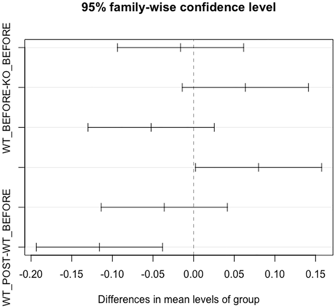
A graph of differences in the mean level of the group versus W T POST - W T BEFORE and W T BEFORE - K O BEFORE. The title reads 95 percent family-wise confidence level. Four lines pass through point 0.00. The first line passes before, and the third line passes after point 0.00.
The 95% family-wise confidence on differences in the mean levels of group
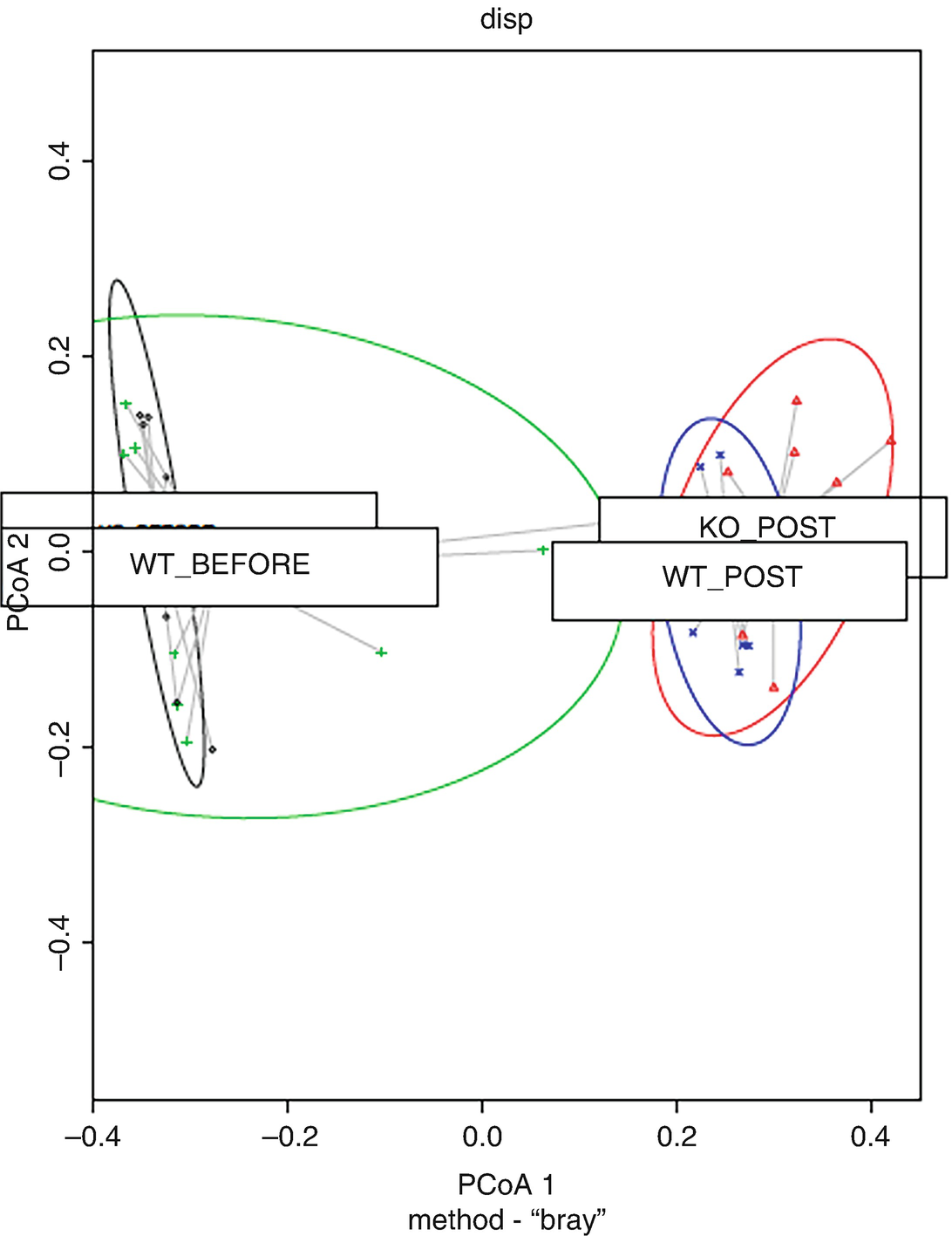
A graph of principal coordinate analysis P C o A 1 versus P C o A 2. There are four ellipses. They are K O BEFORE, W T BEFORE, K O POST, and W T POST. The text below reads method - bray.
Groups and distances to centroids on the first two PCoA axes with data ellipses
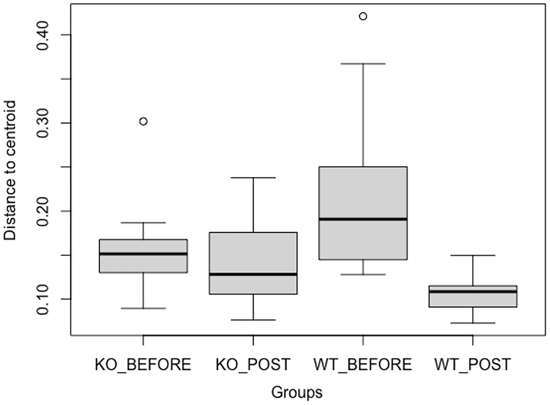
A graph of groups versus distance to the centroid. The groups include K O BEFORE, K O POST, W T BEFORE, and W T POST. The highest point is W T BEFORE. The lowest point is W T POST.
Boxplot of the distances to centroid for each group
11.5 Pairwise PERMANOVA
11.5.1 Introduction to Pairwise PERMMANOVA
In ANOVA and also PERMANOVA, if a null hypothesis of no difference among groups is rejected, then it suggests that there is a significant difference among the defined groups; however, there is no way to know which groups are significantly separated. One way to investigate which groups are different from each other is to conduct pairwise comparisons using an appropriate test and a statistical method to adjust the P-values for multiple comparisons, for example, as we did in Sect. 11.4.2 using permutation test and Tukey’s method. However, the function pairwise.perm.manova() from the RVAideMemoire package (Testing and Plotting Procedures for Biostatistics, version 0.9.81.2 on February 21, 2022, by Maxime Hervé (2022)) is one of specifically designed statistical tools for pairwise comparisons of each group level with corrections for multiple testing after implementing permutational MANOVA. We refer this method as to pairwise PERMMANOVA to represent Pairwise Permutation MANOVA. Several P-value adjustment methods are available for the users to choose, including “bonferroni” (Bonferroni 1936), “holm” (Holm 1979), “hochberg” (Hochberg 1988) and “hommel” (Hommel 1988), “BH” or its alias “FDR” (Benjamini and Hochberg 1995), and “BY” (Benjamini and Yekutieli 2001). Tukey method is not available in this package. Type p.adjust() to check the options and references in R. If you do not want to adjust the P-value, use the pass-through option (“none”).
11.5.2 Implement Pairwise PERMMANOVA Using the RVAideMemoire Package
In this section, we will illustrate how to conduct pairwise comparisons of group using the function pairwise.perm.manova() and how to adjust the P-values for multiple comparisons using various available statistical methods. We will still use the same breast cancer QTRT1 mouse gut microbiome dataset for this illustration. We first need to install and load the RVAideMemoire package:
We then can use either one of the following three sample calls to conduct a pairwise permutational MANOVA:
vegdist(t(otu_tab_rel) is specified to calculate distance matrix; this argument could also be either a typical matrix (one column per variable) or a data frame.
“bray” is specified to calculate Bray-Curtis dissimilarity.
meta_tab_rel$Group4 is a grouping factor variable in meta matrix.
nperm = 999 specifies the number of permutations to obtain the P-value.
test = “Pillai” is used to choose the test statistic when the first argument (e.g., bray) is a matrix.
progress = TRUE or FALSE indicates whether or not display the progress bar.
p.method = “fdr” specifies FDR method for P-value correction. We can choose p.method = “none” to pass through when we do not want to adjust the P-values.
Without adjusting P-values when p.method = “none” is chosen.
Adjust P-values using “fdr” method.
The partial output is given below:
Adjust P-values using “bonferroni” method.
Adjust P-values using “holm” method.
Adjust P-values using “hochberg” method.
Adjust P-values using “hommel” method.
Adjust P-values using “BH” method.
Adjust P-values using “BY” method.
11.6 Identify Core Microbial Taxa Using the Microbiome Package
When a significant association between microbiome abundance and an experiment or biological condition has been detected, microbiome researchers often want to investigate which core or top microbiota (microbial taxa) have contributed to the differences of abundance for further intervention design.
For example, in our study of QTRT1 and gut microbiome in breast cancer (Jilei Zhang et al. 2020), we want to know which top 10 bacteria have contributed to the differences between QTRT1 knockout and wild type as well as before and post treatment.
Step 1: Perform PERMANOVA using the function adonis() and save the modeling results into the object “permanova”.
Step 2: Use the function coefficients() to extract the coefficients of Group4 variable.
By checking the name of Group4 variable of the object “permanova” using head() or tail() function, we know the second column of $model.matrix is named as “Group41”:
Step 3: Plot the top taxa using the barplot() function (Fig. 11.5).
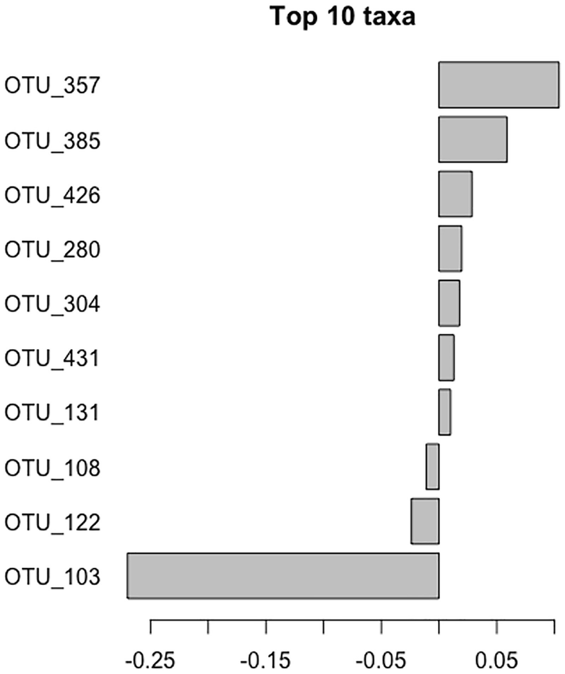
A graph of the top ten taxa. The taxa are O T U underscore 357, O T U underscore 385, O T U underscore 426, O T U underscore 280, O T U underscore 304, O T U underscore 431, O T U underscore 131, O T U underscore 108, O T U underscore 122, and O T U underscore 103.
Top 10 taxa in breast cancer QTRT1 mouse dataset
Top 10 core species identified by PERMANOVA that result in knockout QTRT1 in the MCF7 cells
OTUID | Taxa | Description |
|---|---|---|
OTU_357 | D_5__Lachnospiraceae NK4A136 group | Positive |
OTU_385 | D_4__Lachnospiraceae | Positive |
OTU_426 | D_5_Ruminococcaceae UCG-014 | Positive |
OTU_280 | D_5__Lactobacillus | Positive |
OTU_304 | D_4__Clostridiales vadinBB60 group | Positive |
OTU_431 | D_4__Ruminococcaceae | Positive |
OTU_131 | D_6__Parabacteroides goldsteinii CL02T12C30 | Positive |
OTU_108 | D_5__Alloprevotella | Negative |
OTU_122 | D_5_Alistipes | Negative |
OTU_103 | D_4__Muribaculaceae | Negative |
11.7 Statistical Testing of Beta Diversity in QIIME 2
As we described in Chap. 9, in QIIME 2, diversity analyses are available through the q2-diversity plugin. The analyses include calculating alpha and beta diversity, statistical testing group differences, and generating interactive visualizations. In Chap. 10 (Sect. 10.4), we introduced the calculations of beta diversity measures and the exploration of principal coordinates (PCoA) using emperor plots in QIIME 2. In this section, we introduce statistical testing of beta diversity between group differences in QIIME 2.
In Chap. 9 (Sect. 9.5.1) and Chap. 10 (Sect. 10.4.1), we generated all the alpha diversity and beta diversity measures available in QIIME 2 using a single-command qiime diversity core-metrics-phylogenetic. Here, we repeat this single command as below for recall:
The command generated several beta diversity artifacts including (1) Bray-Curtis distance matrix (bray_curtis_distance_matrix.qza), (2) Jaccard distance matrix (jaccard_distance_matrix.qza), (3) unweighted UniFrac distance matrix (unweighted_unifrac_distance_matrix.qza), and (4) weighted UniFrac distance matrix (weighted_unifrac_distance_matrix.qza). We can use the qiime diversity beta-group-significance command to test the significant differences of beta diversity measures between sample groups.
The beta diversity group significance command generates boxplots of the beta diversity values to visualize the distance between samples aggregated by categorical variables or groups defined in the sample metadata table. It also performs statistical testing of significant differences among groups using the default method PERMANOVA (Anderson 2001) or optional method ANOSIM (Chapman and Underwood 1999). We will perform a statistical testing significant difference in the microbial community beta diversity measures of the time variable in the mouse gut microbiome example.
Different from diversity alpha-group-significance command, which tests for all categorical variables in sample metadata, the diversity beta-group-significance command compares only one sample metadata grouping at a time, so we need to specify the appropriate column name from the sample metadata file to conduct statistical testing.
11.7.1 Significant Testing of Bray-Curtis Distance

A text reads the saved visualization to colon core metrics results forward slash bray Curtis time significance dot q z v.
The above command outputs three results: overview, group significance plots, and pairwise permanova results. The overview results show an all-group PERMANOVA analysis on the Bray-Curtis dissimilarity measures for 2 time groups with sample size 349. The PERMANOVA method performs 999 permutations, resulting pseudo-F test statistic of 38.5453 with P-value of 0.001. Thus the test result reveals that the two time groups have significant differences in their community compositions. The pairwise permanova results show that the pseudo-F test statistic and P-value are the same as the results from overall test since in this case there are only two-group comparisons. The Q-value equals to the P-value of 0.001 since there is no adjustment here.
The raw distance can be downloaded as .tsv file. Two group significance plots are generated including distance to early and distance to late groups and can be saved as PDF format. The pairwise permanova results can be downloaded as CSV format.
11.7.2 Significant Testing of Jaccard Distance
The following qiime diversity beta-group-significance command conducts significant testing of Jaccard distance:

A text reads the saved visualization to colon core metrics results forward slash Jaccard time significance dot q z v.
11.7.3 Significant Testing of Unweighted UniFrac Distance
The following qiime diversity beta-group-significance command conducts significant testing of unweighted UniFrac distance:

A text reads the saved visualization to colon core metrics results forward slash Unweighted UniFrac time significance dot q z v.
11.7.4 Significant Testing of Weighted UniFrac Distance
The following qiime diversity beta-group-significance command conducts significant testing of weighted UniFrac distance:

A text reads the saved visualization to colon core metrics results forward slash Weighted UniFrac time significance dot q z v.
11.8 Summary
Chapter 10 focused on various beta diversity metrics and their calculation as well as exploring them using various ordination techniques. In this chapter, we continued to investigate beta diversity, but focused on statistical hypothesis testing. We first described nonparametric methods for multivariate analysis of variance using permutation tests in ecological and microbiome studies. We then focused on two multivariate nonparametric hypothesis testing methods of beta diversity: ANOSIM and PERMANOVA. We comprehensively described the development of these methods and illustrated their use in microbiome studies through the vegan, phyloseq, and microbiome packages. Followed that, we also illustrated how to analyze multivariate homogeneity of group dispersions, how to conduct pairwise PERMANOVA using the RVAideMemoire package, as well as how to detect core microbial taxa using the microbiome package. Finally, we introduced statistical hypothesis testing for differences of beta diversity between groups in QIIME 2: Bray-Curtis, Jaccard, unweighted UniFrac, and weighted UniFrac distances, respectively.
In Chap. 12, we will introduce the differential abundance analysis of microbiome data using metagenomeSeq.